Field Delineation
Basic info
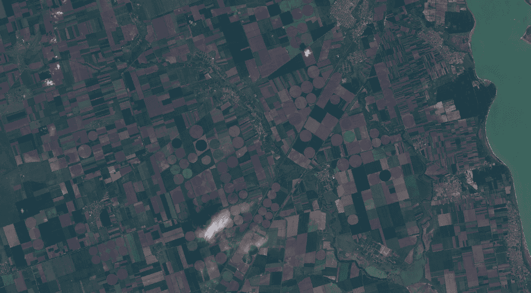
The field delineation marker produces boundaries of the agricultural parcels by clustering the agricultural pixels according to spatial, spectral and temporal properties. The delineated boundaries can aid the farmers speed up the declaration process and the paying agencies to better monitor changes in agricultural use.
| Sentinel-2 | Field delineations |
|---|---|
| 
|
The marker automatically outputs polygon vectors defining agricultural parcels based on Sentinel-2 imagery, although the marker can be seamlessly adapted to work with any remote sensing imagery as an input. The marker was developed as part of the NIVA H2020 project, and thus far has been used for generating parcels for paying agencies, insurance companies and research centres for several regions in Europe and North America.
The marker uses state-of-the-art deep learning (DL) algorithms. The codebase is available in a GitHub repository, and a demo version is available on the Euro Data Cube.
Further info
The marker can be fine-tuned to the users' needs, for instance using existing GSAA datasets to train a deep learning model, or can be used as an off-the-shell algorithm using a deep learning model pre-trained on a different AOI. The marker can estimate parcel boundaries for each cloudless pixel in a Sentinel-2 imagery, and the user can select the time interval over which estimates are aggregated. This approach allows to monitor changes in parcel boundaries, which reflect agricultural activity during the growing season.
In a nutshell, the following steps to produce boundaries of the agricultural parcels are performed:
- split the AOI into a regular grid to speed up processing through massive parallelization
- download remote sensing imagery for the time period of interest;
- (optional) if GSAA data is available, train and evaluate the DL model on reference GSAA and remote sensing imagery;
- predict and post-process agricultural parcel boundaries on remote sensing imagery for the time period of interest.
In case the reference labels are not available, we can also skip step 3 and employ a pre-trained network on data from a different AOI.
Splitting AOI into a grid
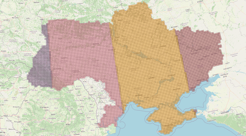
The AOI is split into a regular grid. Each cell, i.e. EOPatch, of the grid has size as we find appropriate, and overlaps with the neighbouring cell a given amount of pixels. Splitting into cells allows to massively parallelize the processing, and the overlap ensures that the results are merged seamlessly. On the image below: Ukraine split into tiles of 10km x 10km, tiles are in their own UTM zone.
Data download
For the selected time periods, remote sensing images are downloaded for each EOPatch as well as the cloud masks. Data downloading is executed using Sentinel Hub Batch Processing API.
Analysis of cloud and snow coverage
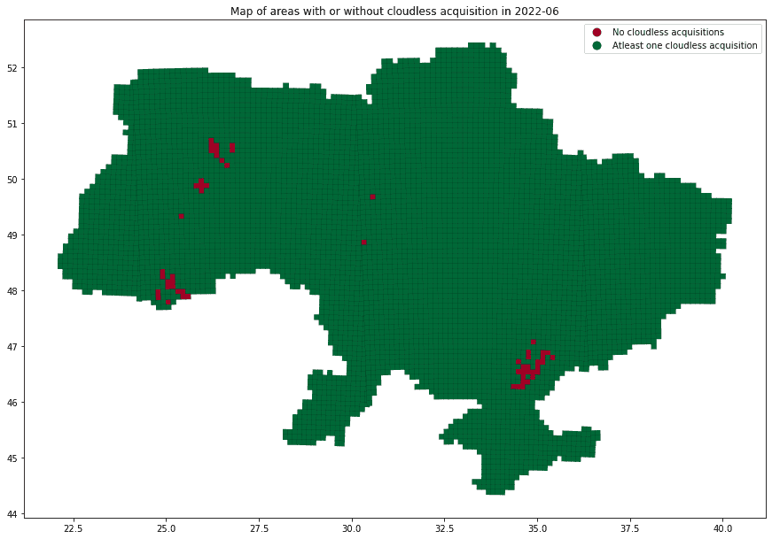
Once the remote sensing imagery and cloud masks are available for each EOPatch, statistics over the available months are computed to estimate how many cloudless scenes are available. Our field delineation algorithm produces estimates for each available acquisition, however, only fields estimated for acquisitions with cloud and snow coverage below 5% of area of the EOPatch are typically kept and a consensus generated. This is performed in order to ensure that clouds and other artefacts don't affect the estimation of boundaries. On the image below: invalid observations over a month.
Reference data and sampling (optional)
GSAA vectors are a great reference data for training of the ML model: for a given year, the majority of the GSAA parcels correctly match the agricultural land cover, with the exception of a minority of incorrect parcels resulting from outdated information or incorrect applications. If available, these vectors can be used to fine-tune the marker to improve its parcel boundary estimation.
The GSAA along with the remote sensing imagery is further sampled into smaller patchlets to speed up the training of the deep learning model. Using sampling, a constraint can be made on the minimal area covered by the reference GSAA in each sample, allowing to control the amount of positive and negative examples the model sees.
Normalization
As we want our model to perform well over timestamps taken over the whole year, it’s very important how the data is normalized. For each individual patchlet timestamp, statistics that could be used for normalization are calculated for each band. As well as computing overall statistics, we evaluate these temporally to establish whether a single or multiple normalization factors for the time period of interest are needed. We look at mean, standard deviation and quantiles for each month.
As mentioned above, in case the reference labels are not available to fine-tune our deep learning algorithm, we use an existing model trained on data in another AOI. In this case, a key factor to achieve meaningful results is to adequately normalize the input reflectance values, so that the input distributions for the area of interest (where the boundaries are predicted) are as aligned as possible to the reflectance distributions the model has seen during training.
Semantic segmentation
We apply semantic segmentation on each single-scene separately, and combine predictions temporally at a later stage. A model trained this way should learn to be invariant to the time-period of interest. The aim of the parcel delineation in CAP practices is generally to monitor agricultural land cover throughout the growing season, but the beginning of the season is of particular interest as is typically the time the farmers fill in their applications. A model that can generalise to different time periods seems therefore useful in this perspective, and that justifies our choice of training a single-scene model and combining temporally the predictions in a second stage.
Temporal merging
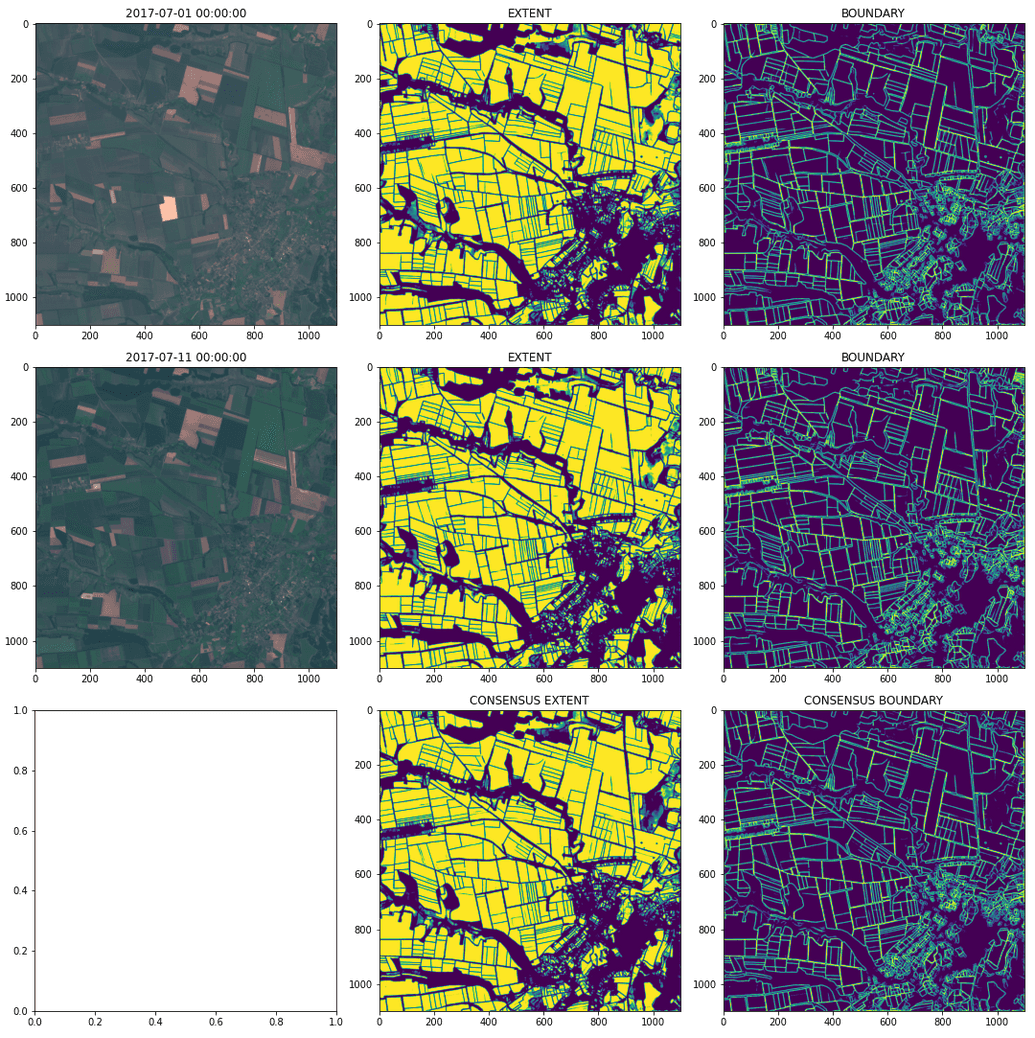
Once the model estimates field boundaries, e.g. extent and boundary masks, for each timestamp for each EOPatch, these are temporally and spatially merged to derive a single probability map, which is then contoured to obtain the final vector polygons. The temporal merging generates a consensus of extent and boundary masks over a given time period (see example on figure below).
Contouring
The consensus raster extent and boundary masks for the chosen time period are spatially merged and contoured to derive enclosed vector polygons. Parameters for the contouring can be optimised to control the appearance of the final polygons.
Shape attributes
For each estimated polygon, we compute its area, circumference, shapeness and circumference/area (CA) ratio. Shapeness calculates the Hausdorff distance between the polygon and its minimum rotated rectangle, while the CA ratio provides an indication of the regularity of the polygon. These attributes can be used to further filter out polygons which are likely not cultivated, e.g. with large areas and large values of shapeness (see some examples in the figure below).
Dynamic analysis
The field delineation marker can be computed for different time periods, and the resulting polygons can be used to track and monitor agricultural activity. For instance, estimated parcels derived early in the season can be compared to parcels estimated at peak growing season, providing insights into whether the field boundaries changed or not.
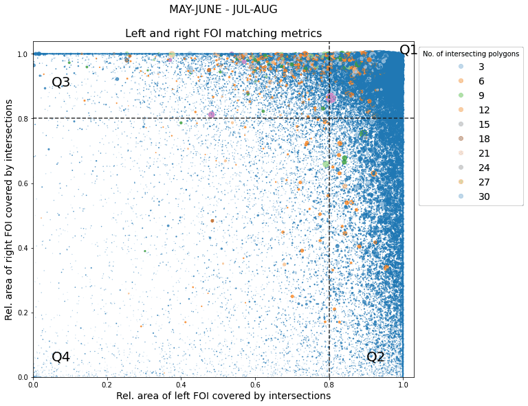
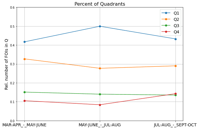
The figures below show such a comparison, and the quantitative metrics that quantify changes in field contours, that can be further used to monitor agricultural activity.
The quantitative metrics can be computed for each estimated field, and used to derive overall insights into the performance of the marker, as well as into the changes due agricultural activity, as shown below. These plots show that parcels tend to change more at the beginning and end of the growing season, e.g. from March to May and from August to October, due to ploughing and harvesting activities which can reduce the visibility of boundaries. Estimated parcels show less changes and are possibly more accurate at the peak of the growing season, e.g. from May to July.
|
|
Links
Webinar: Automated Agricultural Field Delineation Tool
Blog post about Parcel boundary detection for CAP
Interactive interface for viewing delineated fields in Lithuania for June 2020
